Tutorials

There are two main ways of accessing the resources of the stdpopsim package that will be detailed in this tutorial. The first is via the command line interface (CLI). This is useful if you want to do a straightforward run of the models in the stdpopsim Catalog. The other way to access the stdpopsim resources is via the Python API. This is a bit more complicated, but allows for more advanced tasks. This tutorial will walk through both ways of using the stdpopsim package as well as a few examples of producing and processing output.

To simulate genomes using stdpopsim, we need to make several choices about what will be simulated:

which species
which contig (i.e., how much of what chromosome)
which recombination/genetic map
which demographic model
how many samples from each population of the model
whether to simulate selection (via a distribution of fitness effects), and if so where to introduce selected mutations (i.e. in an exon annotation track)
which simulation engine to use

These choices are nested: the species determines what contigs, recombination/genetic maps, and demographic models are available, and the demographic model determines how many populations can be sampled from. Currently, the two choices of simulation engine are msprime and SLiM, and incorporating selection into simulations is only possible using the SLiM engine. Below are examples of making these choices in various contexts, using both CLI and Python interfaces.

Note

Recombination map and genetic map are terms used to describe maps of recombination rates that vary across and along chromosomes. In the stdpopsim code and documentation, we use the term genetic map to refer specifically to a “crossing-over rate map” and recombination map to refer to a “crossing-over and gene conversion rate map.”” See further details on this distinction.

Running stdpopsim with the command-line interface (CLI)

In order to use the stdpopsim CLI the stdpopsim package must be installed (see Installation). The CLI provides access to the Catalog of models that have already been implemented by stdpopsim.

A first simulation

As a first step, we’ll use the CLI built-in help to build up to a realistic coalescent simulation of some copies of human chromosome 22 with the HapMap genetic map, and a published demographic model.

Choose a species and a contig

The first step for using the CLI is to select the species that you are interested in simulating data for. In order to see which species are available run

$ stdpopsim --help
usage: stdpopsim [-h] [-V] [-v | -q] [-c CACHE_DIR] [-e {msprime,slim}]
                 [--msprime-model {hudson,dtwf,smc,smc_prime}]
                 [--msprime-change-model T MODEL] [--slim-path PATH]
                 [--slim-script] [--slim-scaling-factor Q] [--slim-burn-in X]
                 {AedAeg,AnaPla,AnoCar,AnoGam,ApiMel,AraTha,BosTau,CaeEle,CanFam,ChlRei,DroMel,DroSec,EscCol,GasAcu,GorGor,HelAnn,HelMel,HomSap,MusMus,OrySat,PanTro,PapAnu,PhoSin,PonAbe,RatNor,StrAga,SusScr,download-genetic-maps}
                 ...

Command line interface for stdpopsim.

positional arguments:
  {AedAeg,AnaPla,AnoCar,AnoGam,ApiMel,AraTha,BosTau,CaeEle,CanFam,ChlRei,DroMel,DroSec,EscCol,GasAcu,GorGor,HelAnn,HelMel,HomSap,MusMus,OrySat,PanTro,PapAnu,PhoSin,PonAbe,RatNor,StrAga,SusScr,download-genetic-maps}
    AedAeg              Run simulations for Aedes aegypti.
    AnaPla              Run simulations for Anas platyrhynchos.
    AnoCar              Run simulations for Anolis carolinensis.
    AnoGam              Run simulations for Anopheles gambiae.
    ApiMel              Run simulations for Apis mellifera.
    AraTha              Run simulations for Arabidopsis thaliana.
    BosTau              Run simulations for Bos taurus.
    CaeEle              Run simulations for Caenorhabditis elegans.
    CanFam              Run simulations for Canis familiaris.
    ChlRei              Run simulations for Chlamydomonas reinhardtii.
    DroMel              Run simulations for Drosophila melanogaster.
    DroSec              Run simulations for Drosophila sechellia.
    EscCol              Run simulations for Escherichia coli.
    GasAcu              Run simulations for Gasterosteus aculeatus.
    GorGor              Run simulations for Gorilla gorilla.
    HelAnn              Run simulations for Helianthus annuus.
    HelMel              Run simulations for Heliconius melpomene.
    HomSap              Run simulations for Homo sapiens.
    MusMus              Run simulations for Mus musculus.
...

This shows the species currently supported by stdpopsim. This means that stdpopsim knows various traits of these species, including chromosome size, recombination rate(s), etc. Once we’ve selected a species, in this case humans, we can look at the help again as follows.

$ stdpopsim HomSap --help
usage: stdpopsim HomSap [-h] [--help-models [HELP_MODELS]] [-b BIBTEX_FILE]
                        [--help-genetic-maps [HELP_GENETIC_MAPS]] [-D] [-g]
                        [--help-dfes [HELP_DFES]] [-c] [-L LENGTH]
                        [-i INCLUSION_MASK] [-e EXCLUSION_MASK]
                        [-l LENGTH_MULTIPLIER] [--left LEFT] [--right RIGHT]
                        [-s SEED] [--keep-mutation-ids-as-alleles] [-d]
                        [--dfe] [--dfe-interval] [--dfe-bed-file]
                        [--help-annotations [HELP_ANNOTATIONS]]
                        [--dfe-annotation] [-o OUTPUT]
                        samples [samples ...]

Run simulations for Homo sapiens using up-to-date genome information,
genetic maps and simulation models from the literature. NOTE: By
default, the tskit '.trees' binary file is written to stdout,so you
should either redirect this to a file or use the '--output' option to
specify a filename.

Default population parameters for Homo sapiens:
Generation time: 30
Population size: 10000
...

For conciseness we do not show all the output here but this time you should see a different output which shows options for performing the simulation itself and the species default parameters. This includes selecting the demographic model, chromosome, genetic map, distribution of fitness effects, and number of samples.

The most basic simulation we can run is to simulate a diploid genome - i.e., a single individual - using the species’ defaults as seen in the species help (stdpopsim HomSap --help). These defaults include constant size population named pop_0, a uniform genetic map based on the average recombination rate (either genome-wide or within a chromosome, if specified), and the mutation rate shown above. To save time we will specify that the simulation use chromosome 22, using the -c option. We also specify that the resulting tree-sequence formatted output should be written to the file foo.ts with the -o option. For more information on how to use tree-sequence files see tskit. Finally, we specify that a single (diploid) sample should be simulated for population pop_0 using the syntax <population_name>:<number_of_samples>.

$ stdpopsim HomSap -c chr22 -o foo.ts pop_0:1

Warning

It’s important to remember to either redirect the output of stdpopsim to file or to use the -o/--output option. If you do not, the binary output may mess up your terminal session.

Choose a model and a sampling scheme

Next, suppose we want to use a specific demographic model. We look up the available models using the --help-models flag (here, truncated for space):

$ stdpopsim HomSap --help-models

All simulation models for Homo sapiens

Africa_1B08: African-americans population
     African-American two-epoch instantaneous growth model from Boyko
    et al 2008, fit to the synonymous SFS for the 11 of 15 African
    Americans showing the least European ancestry, using coalescent
    simulations with recombination with the maximum likelihood method
    of Williamson et al 2005; times were calibrated assuming 3e5
    generations since human-chimp divergence and fitting the number of
    synonymous human-chimp differences. Mutation and recombination
    rates were assumed to be the same (1.8e-8).

    Populations:
        African_Americans: African-Americans from Boyko et al 2008

Africa_1T12: African population
     The model is a simplification of the two population Tennesen et
    al. model with the European-American population removed so that we
    are modeling the African population in isolation.

    Populations:
        AFR: African

AmericanAdmixture_4B18: American admixture
     Demographic model for American admixture, taken from Browning et
    al. 2018. This model extends the Gravel et al. (2011) model of
    African/European/Asian demographic history to simulate an admixed
    population with admixture occurring 12 generations ago. The
    admixed population had an initial size of 30,000 and grew at a
...

This gives all of the possible demographic models we could simulate. We choose the two-population out-of-Africa model from Tennesen et al. (2012) . By looking at the output from --help-models we find that the name for this model is OutOfAfrica_2T12 and that we can specify it using the --demographic-model/-d option. We choose to draw two diploid sample from the AFR (“African American”) population, and three diploids from the EUR (“European American”) population. To increase simulation speed we can also choose to simulate a subset of the chromosome via the --left and --right options. If we were using a genetic map and/or annotation track, these would be clipped to the contig boundaries. The command now looks like this:

$ stdpopsim HomSap -c chr22 --left 10000000 --right 20000000 -o foo.ts -d OutOfAfrica_2T12 AFR:2 EUR:3

Note that the number of samples from each population are simply specified as <population_name>:<number_of_samples> at the end of the command. Omitted populations will have no samples in the resulting tree sequence.

Note

Many demographic models were inferred or calibrated using a mutation rate or recombination rate that differs from the cataloged species’ rate. Simulations using the CLI now automatically use the model’s specified mutation rate or recombination rate instead of the species rate, so that expected levels of diversity more closely match those observed in the data that were used to infer the demographic model. For generic demographic models or those without associated mutation or recombination rates, the species rates are used.

Now we want to add an empirical genetic map to make the simulation more realistic. We can look up the available genetic maps using the --help-genetic-maps flag (here, truncated for space):

$ stdpopsim HomSap --help-genetic-maps

All genetic maps for Homo sapiens

DeCodeSexAveraged_GRCh36
     This genetic map is from the deCode study of recombination events
    in 15,257 parent-offspring pairs from Iceland. 289,658 phased
    autosomal SNPs were used to call recombinations within these
    families, and recombination rates computed from the density of
    these events. This is the combined male and female (sex averaged)
    map. See https://www.decode.com/addendum/ for more details.

DeCodeSexAveraged_GRCh38
     This genetic map is from the deCode study of recombination events
    in 15,257 parent-offspring pairs from Iceland. 289,658 phased
    autosomal SNPs were used to call recombinations within these
    families, and recombination rates computed from the density of
    these events. This is the combined male and female (sex averaged)
    map. See https://www.decode.com/addendum/ for more details. This
    map is further lifted over from the original GRCh36 to GRCh38
    using liftover. Liftover was performed using the
...

In this case we choose the HapMapII_GRCh38 map and simulate the entire chromosome.

$ stdpopsim HomSap -g HapMapII_GRCh38 -c chr22 -o foo.ts -d OutOfAfrica_2T12 AFR:2 EUR:3

For reproducibility we can also choose set the seed for the simulator using the -s flag.

$ stdpopsim HomSap -s 1046 -g HapMapII_GRCh38 -c chr22 -o foo.ts \
$    -d OutOfAfrica_2T12 AFR:2 EUR:3

On running these commands, the CLI also outputs the relevant citations for both the simulator used and the resources used for simulation scenario.

Convert output to VCF

The output from a stdpopsim simulation is a tree sequence, a compact and efficient format for storing both genealogies and genome sequence. Some examples of analyzing tree sequences are given below. If desired, these can be converted to VCF on the command line if the tskit package is installed, with the tskit vcf command:

$ tskit vcf foo.ts > foo.vcf

For this small example (only five diploid samples), the file sizes are similar, but the tree sequence is slightly larger than the VCF (it does carry a good bit more information about the trees, after all). However, if we up the sample sizes to 1000 and 1500 (the simulation is still pretty quick) the tree sequence is fifty-two times smaller:

$ stdpopsim HomSap -s 1046 -g HapMapII_GRCh38 -c chr22 -o foo.ts \
$    -d OutOfAfrica_2T12 AFR:1000 EUR:1500
$ tskit vcf foo.ts > foo.vcf
$ ls -lth foo.*
-rw-rw-r-- 1 natep natep 8.6G Oct  4 12:03 foo.vcf
-rw-rw-r-- 1 natep natep 163M Oct  4 12:02 foo.ts

Zipping the files (using the tszip package) reduces this difference quite a lot, but increases time required for processing:

$ tskit vcf foo.ts | gzip -c > foo.vcf.gz
$ tszip foo.ts
$ ls -lth foo.*
-rw-rw-r-- 1 natep natep  49M Oct  4 12:06 foo.ts.tsz
-rw-rw-r-- 1 natep natep 103M Oct  4 12:05 foo.vcf.gz

Using the `SLiM` simulation engine

The default “simulation engine” - i.e., the program that actually does the simulating - is msprime, a coalescent simulator. However, it is also possible to swap this out for SLiM, a forwards-time, individual-based simulator.

Specifying the engine

Using SLiM is as easy as passing the --engine/-e flag (we didn’t do this above, so it used the default engine, msprime). For instance, to use SLiM to simulate the same chunk of chromosome 22 under the OutOfAfrica_2T12 model as above, we would just run:

$ stdpopsim -e slim HomSap -c chr22 --left 10000000 --right 20000000 \
$    -o foo.ts -d OutOfAfrica_2T12 AFR:1 EUR:2

But: this simulation can take quite a while to run, so before you try that command out, read on!

`SLiM` scaling factor

The previous example is a pretty big simulation, even with only a portion of a chromosome, due to the large number of individuals (unlike msprime, SLiM must actually simulate all the individuals in the population, regardless of the number of samples). To make it run fast enough for a tutorial, we can specify a scaling factor (\(Q\)) using the --slim-scaling-factor option. Unlike the previous command, this one should run very fast:

$ stdpopsim -e slim --slim-scaling-factor 10 HomSap -c chr22 \
$    --left 10000000 --right 20000000 -o foo.ts -d OutOfAfrica_2T12 AFR:1 EUR:2

This example runs in less than a minute, wheras without setting the scaling factor it takes the same computer upwards of 20 minutes. Briefly, this speedup is accomplished by reducing all of the population sizes by a “scaling factor” (here set to 10), and rescaling time by the same factor (thus increasing mutation, recombination, and population growth rates). A model with selection would also need to rescale selection coefficients by the same factor. This results in simulations that are equivalent in many senses – the same rate of genetic drift, the same expected decay of linkage disequilibrium – but generally run much faster because there are fewer individuals to keep track of. In practice, rescaling seems to produce indistinguishable results in much shorter times at many parameter values. However, the user should be aware that in principle, the results are not equivalent, possibly in subtle and hard-to-understand ways. This is particularly true in simulations with large amounts of selection. See the SLiM manual and/or Urrichio & Hernandez (2014) for more discussion.

Simulating genomes with selection

The examples above simulate contigs given a species, a genetic map, and a demographic model; but assume that all genetic variation is neutral (has no impact on fitness). It is possible to incorporate selection in the simulations by (1) specifying the Distribution of Fitness Effects (DFE) for all new mutations across the entire contig or a subset of it; or by (2) adding a single mutation under selection, as for instance in a selective sweep.

If a DFE is already described in the catalog, one can incorporate it into the simulation with the flag --dfe. For instance, HomSap has a DFE named Gamma_K17. To add it the example above, we can use the command:

$ stdpopsim -e slim --slim-scaling-factor 20 HomSap -c chr22 \
$    --left 10000000 --right 20000000 --dfe Gamma_K17 \
$    -o foo.ts -d OutOfAfrica_2T12 AFR:1 EUR:2

which will introduce selected and neutral mutations following the proportions described in Gamma_K17.

Instead of simulating a DFE that convers the entire contig, one can simulate only coding sequence (CDS) by using the flag --dfe-annotation and specifying a CDS annotation:

$ stdpopsim -e slim --slim-scaling-factor 20 HomSap -c chr22 \
$    --left 10000000 --right 20000000 --dfe Gamma_K17 \
$    --dfe-annotation ensembl_havana_104_CDS \
$    -o foo.ts -d OutOfAfrica_2T12 AFR:1 EUR:2

If instead of an bundled annotation, one has a bed file (e.g. ex.bed) like the one below:

$ cat ex.bed
chr1  10000000  14500000
chr1  15000000  30002425
chr1  30002430  30003000

then a DFE may be applied to all intervals in the bed file by using the option --dfe-bed-file:

$ stdpopsim -e slim --slim-scaling-factor 20 HomSap -c chr22 \
$    --left 10000000 --right 20000000 --dfe Gamma_K17 \
$    --dfe-bed-file ex.bed -o foo.ts -d OutOfAfrica_2T12 AFR:1 EUR:2

To apply a DFE to a small portion of a contig, the option --dfe-interval <start>,<end> may be used:

$ stdpopsim -e slim --slim-scaling-factor 20 HomSap -c chr22 \
$    --left 10000000 --right 20000000 --dfe Gamma_K17 \
$    --dfe-interval 14001000,14005000 -o foo.ts -d OutOfAfrica_2T12 AFR:1 EUR:2

The examples above (using --dfe-bed-file and --dfe-interval) model selection on specified genomic intervals that also fall within the region being simulated (10 Mb to 20 Mb on chr22). In other words, the supplied DFE intervals are clipped to the contig endpoints on the chromosome. For example, the third interval in ex.bed above will be silently omitted from the simulation.

Warning

Simulating a region under selection is not the same as simulating a chromosome under selection and clipping to the region. This is because selected mutations outside of the region can influence ancestry within the region, due to linkage.

See also the Python API to incorporate selection.

Debugging output from `SLiM`

Next we’ll look at running a different model with SLiM, but with some sanity checks along the way.

Choose a species: Drosophila melanogaster

Perusing the Catalog, we see that to simulate copies of chromosome arm 2L from Drosophila melanogaster individuals with the demographic model inferred by Sheehan & Song (2016), using SLiM with a (very extreme) scaling factor of 1000, we could run

$ stdpopsim -e slim --slim-scaling-factor 1000 DroMel -c chr2L \
$    --right 1000000 -o foo.ts -d African3Epoch_1S16 AFR:50

The scaling factor of 1000 makes this model run very quickly, but should also make you very nervous. What actually is being simulated here? We can at least find out what the actual population sizes are in the SLiM simulation by asking the simulation to be more verbose. Prepending the -vv flag will request that SLiM print out information every time a demographic event occurs (helpfully, this also gives us an idea of how quickly the simulation is going):

$ stdpopsim -vv -e slim --slim-scaling-factor 1000 DroMel -c chr2L \
$    --right 1000000 -o foo.ts -d African3Epoch_1S16 AFR:50 \
$    | grep "^DEBUG:"
DEBUG: Making flat contig of length 1000000 from 2L
DEBUG: // Initial random seed:
DEBUG: 2214454132353
DEBUG:
DEBUG: // RunInitializeCallbacks():
DEBUG: initializeMutationType(0, 0.5, "f", 0);
DEBUG: initializeGenomicElementType(0, m0, 1);
DEBUG: initializeGenomicElement(g0, 0, 999999);
DEBUG: initializeMutationRate(0, 999999);
DEBUG: initializeTreeSeq();
DEBUG: initializeRecombinationRate(2.40457e-05, 999999);
DEBUG:
DEBUG: // Starting run at tick <start>:
DEBUG: 1
DEBUG:
DEBUG: 1: p = sim.addSubpop(0, 652);
DEBUG: 1: p.name = 'AFR';
DEBUG: 1: Starting burn-in...
DEBUG: 6521: {p0.setSubpopulationSize(145);}
DEBUG: 8521: {p0.setSubpopulationSize(544);}
DEBUG: 8721: {inds=p0.sampleIndividuals(50); sim.treeSeqRememberIndividuals(inds);}
DEBUG: 8721: {end();}
...

This tells us that after rescaling by a factor of 1000, the population sizes in the three epochs are 652, 145, and 544 individuals, respectively. No wonder it runs so quickly! At the end, fifty (diploid) individuals are sampled. These numbers are not obviously completely wrong, as would be for instance if we had population sizes of 1 or 2 individuals. However, extensive testing would need to be done to find out if data produced with such an extreme scaling factor actually resembles the data that would be produced without rescaling.

Running stdpopsim with the Python interface (API)

Nearly all the functionality of stdpopsim is available through the CLI, but for complex situations it may be desirable to use Python. Furthermore, downstream analysis may happen in Python, using the tskit tools for working with tree sequences. In order to use the stdpopsim API the stdpopsim package must be installed (see Installation).

Running a published model

The first example uses a mostly default genome with a published demographic model.

Pick a species and demographic model

First, we will pick a species (here, humans) and the published demographic model to simulated under. In stdpopsim there are two types of model: ones taken to match the demographic history reported in published papers, and “generic” models. We’ll first simulate using a published model from the catalog. Let’s see what demographic models are available for humans:

import stdpopsim

species = stdpopsim.get_species("HomSap")

for x in species.demographic_models:
    print(x.id)

# OutOfAfricaExtendedNeandertalAdmixturePulse_3I21
# OutOfAfrica_3G09
# OutOfAfrica_2T12
# Africa_1T12
# AmericanAdmixture_4B18
# OutOfAfricaArchaicAdmixture_5R19
# Zigzag_1S14
# AncientEurasia_9K19
# PapuansOutOfAfrica_10J19
# AshkSub_7G19
# OutOfAfrica_4J17
# Africa_1B08
# AncientEurope_4A21

These models are described in detail in the Catalog. We’ll look at the first model, OutOfAfrica_3G09, from Gutenkunst et al (2009). We can check how many populations exist in this model, and what they are:

model = species.get_demographic_model("OutOfAfrica_3G09")
print(model.num_populations)
# 3
print(model.num_sampling_populations)
# 3
print([pop.name for pop in model.populations])
# ['YRI', 'CEU', 'CHB']

This model has 3 populations, named YRI, CEU, CHB, and all three can be sampled from. The number of “sampling” populations could be smaller than the number of populations, since some models have ancient populations which are currently not allowed to be sampled from – but that is not the case in this model.

If working in a notebook, it’s also possible to plot a schematic of your chosen model using the demesdraw python library. This provides both a size_history plot and a tubes visualization. E.g.

import demesdraw

graph = model.model.to_demes()
demesdraw.tubes(model.model.to_demes())

Equivalent plots for all the available demographic models are also shown in the Catalog.

Set up the contig

We’ll next define the contig, which contains information about the genome length we want to simulate and recombination and mutation rates. Here, we use the human chromosome 22. If no genetic map is specified, we assume a uniform recombination rate set to the average recombination rate for that chromosome.

contig = species.get_contig("chr22")

# default is a uniform genetic map
print("mean recombination rate:", f"{contig.recombination_map.mean_rate:.3}")
# mean recombination rate: 2.11e-08

# and the default mutation rate is based on the species default
print("mean mutation rate:", contig.mutation_rate)
# mean mutation rate: 1.29e-08

# but note that the mutation rate differs from the model's assumed rate
print("model mutation rate:", model.mutation_rate)
# model mutation rate: 2.35e-08

The Gutenkunst OOA model was inferred using a mutation rate much larger than the default mutation rate for humans in the stdpopsim catalog. As such, simulating using this model and default rate will result in levels of diversity substantially lower than expected for the human population data that this model was inferred from. To match observed diversity in humans, we should instead use the mutation rate associated with the demographic model:

contig = species.get_contig("chr22", mutation_rate=model.mutation_rate)
print(contig.mutation_rate == model.mutation_rate)
# True

Similar functionality exists for the recombination rate, if a model specifies one.

Choose a sampling scheme and simulate

The final ingredient we need before simulating is a specification of the number of samples from each population. We’ll simulate 5 diploids each from YRI and CHB, and zero from CEU, using msprime as the simulation engine:

samples = {"YRI": 5, "CHB": 5, "CEU": 0}
engine = stdpopsim.get_engine("msprime")
ts = engine.simulate(model, contig, samples)
print(ts.num_sites)
# 152582

And that’s it! It’s that easy! We now have a tree sequence describing the history and genotypes of 20 haploid genomes, between which there are 152,582 variant sites. (We didn’t set the random seed, though, so you’ll get a somewhat different number.)

Let’s look at the metadata for the resulting simulation, to make sure that we’ve got what we want.

ts.num_samples
# 20

for k, pop in enumerate(ts.populations()):
    print(
        f"The tree sequence has {len(ts.samples(k))} samples from "
        f"population {k}, which is {pop.metadata['id']}."
    )
# The tree sequence has 10 samples from population 0, which is YRI.
# The tree sequence has 0 samples from population 1, which is CEU.
# The tree sequence has 10 samples from population 2, which is CHB.

Running a generic model

Next, we will simulate using a “generic” model, with piecewise constant population size. This time, we will simulate a given genome length under a uniform genetic map, using an estimate of the human effective population size from the Catalog.

Choose a species

Although the model is generic, we still need a species in order to get the contig information. Again, we’ll use Homo sapiens, which has the id “HomSap”. (But, you could use any species from the Catalog!)

import stdpopsim

species = stdpopsim.get_species("HomSap")

Set up the generic model

Next, we set the model to be the generic piecewise constant size model, using the predefined human effective population size (see Catalog). Since we are providing only one effective population size, the model is a single population of constant over all time.

model = stdpopsim.PiecewiseConstantSize(species.population_size)

Each species has a “default” population size, species.population_size, which for humans is 10,000.

Choose a contig and genetic map

Next, we set the contig information. Again, we could use any of the chromosomes listed in the Catalog (or a fraction of a chromosome, using the left and right arguments), keeping in mind that larger contigs will take longer to simulate. We could also specify a “generic” contig, which provides a segment of a given length with constant recombination rate, taken to be the average rate over all chromosomes for that species. Here, we define a contig of length 1 Mb:

contig = species.get_contig(length=1e6)
print(contig.recombination_map.sequence_length)
# 1000000.0
print(contig.recombination_map.mean_rate)
# 1.2820402396300886e-08
print(contig.mutation_rate)
# 1.29e-8

The “sequence length” is the length in base pairs. Since we are using a generic contig, we cannot specify a genetic map so we get a uniform map with a constant recombination rate. The mutation rate defaults to the species average mutation rate, as no mutation rate was provided when defining the contig.

Choose a sampling scheme, and simulate

Next, we set the number of samples and set the simulation engine. In this case we will simulate genomes of 5 diploids using the simulation engine msprime (note that the generic PiecewiseConstantSize model has a single population named pop_0). But, you can go crazy with the sample size! msprime is great at simulating large samples!

samples = {"pop_0": 5}
engine = stdpopsim.get_engine("msprime")

Finally, we simulate the model with the contig length and number of samples we defined above. The simulation results are recorded in a tree sequence object (tskit.TreeSequence).

ts = engine.simulate(
    model, contig, samples, msprime_model="dtwf", msprime_change_model=[(20, "hudson")]
)

The msprime_model argument is optional; it specifies that the most recent 20 generations be simulated with the discrete time Wright-Fisher (“dtwf”) model (followed by a switch to the more efficient “hudson” coalescent model). This is good practice for large samples, for which the Hudson model can be an inaccurate approximation for the most recent few generations.

Sanity check the tree sequence output

Now, we do some simple checks that our simulation worked with tskit.

print(ts.num_samples)
# 10
print(ts.num_populations)
# 1
print(ts.num_mutations)
# 1322
print(ts.num_trees)
# 1021

As expected, there are 10 haploids in one population. We can also see that it contains 1021 distinct genealogical trees across this 1Mb of sequence, on which there were 1322 mutations (since we are not using a seed here, the number of mutations and trees will be slightly different for you). Try running the simulation again, and notice that the number of samples and populations stays the same, while the number of mutations and trees changes.

Output to VCF

In addition to working directly with the simulated tree sequence, we can also output other common formats used for population genetics analyses. We can use tskit to convert the tree sequence to a vcf file called “foo.vcf”. See the tskit documentation (tskit.TreeSequence.write_vcf()) for more information.

with open("foo.vcf", "w") as vcf_file:
    ts.write_vcf(vcf_file, contig_id="0")

Taking a look at the vcf file, we see something like this:

##fileformat=VCFv4.2
##source=tskit 0.5.0
##FILTER=<ID=PASS,Description="All filters passed">
##contig=<ID=0,length=1000000>
##FORMAT=<ID=GT,Number=1,Type=String,Description="Genotype">
#CHROM      POS     ID      REF     ALT     QUAL    FILTER  INFO    FORMAT  tsk_0   tsk_1   tsk_2   tsk_3   tsk_4
0   511     0       G       A       .       PASS    .       GT      0|0     0|0     0|0     1|1     0|0
0   930     1       A       C       .       PASS    .       GT      0|0     0|0     0|0     0|0     0|1
0   1209    2       T       A       .       PASS    .       GT      0|0     0|0     0|0     0|1     0|0
0   1308    3       T       G       .       PASS    .       GT      0|0     0|1     0|0     0|0     0|0
0   2271    4       A       C       .       PASS    .       GT      1|0     0|1     1|0     0|0     0|0
0   2637    5       C       T       .       PASS    .       GT      1|0     0|1     1|1     0|0     0|0
0   3615    6       G       A       .       PASS    .       GT      0|0     0|0     0|0     0|0     1|0
0   4391    7       G       T       .       PASS    .       GT      0|1     1|0     0|0     1|1     1|1
...

Using the `SLiM` engine

Above, we used the coalescent simulator msprime as the simulation engine, which is in fact the default. However, stdpopsim also has the ability to produce simulations with SLiM, a forwards-time, individual-based simulator. Using SLiM provides us with a few more options. You may also want to install the pyslim package to extract the additional SLiM-specific information in the tree sequences that are produced.

An example simulation

The stdpopsim tool is designed so that different simulation engines are more or less exchangeable, so that to run an equivalent simulation with SLiM instead of msprime only requires specifying SLiM as the simulation engine. Here is a simple example.

Choose the species, contig, and genetic map

First, let’s set up a simulation of 10 Mb of human chromosome 22 with a uniform genetic map, drawing 100 diploids from the Tennesen et al (2012) model of African history, Africa_1T12 (which has a single population named AFR). Since SLiM must simulate the entire population, sample size does not affect the run time of the simulation, only the size of the output tree sequence (and, since the tree sequence format scales well with sample size, it doesn’t affect this very much either).

import stdpopsim

species = stdpopsim.get_species("HomSap")
model = species.get_demographic_model("Africa_1T12")
contig = species.get_contig(
    "chr22", left=10e6, right=20e6, mutation_rate=model.mutation_rate
)
# default is a uniform genetic map with average rate across chr22
samples = {"AFR": 100}

Choose the simulation engine

This time, we choose the SLiM engine, but otherwise, things work pretty much just as before.

engine = stdpopsim.get_engine("slim")
ts = engine.simulate(model, contig, samples, slim_scaling_factor=10)

(Note: you have to have SLiM installed for this to work, and if it isn’t installed in your PATH, so that you can run it by just typing slim on the command line, then you will need to specify the slim_path argument to simulate.) To get an example that runs quickly, we have set the scaling factor, described in more detail below (SLiM scaling factor),

Other `SLiM` options

Besides rescaling, there are a few additional options specific to the SLiM engine, discussed here.

The `SLiM` burn-in

Another option specific to the SLiM engine is slim_burn_in: the amount of time before the first demographic model change that SLiM begins simulating for, in units of \(N\) generations, where \(N\) is the population size at the first demographic model change. By default, this is set to 10, which is fairly safe. History before this period is simulated with an msprime coalescent simulation, called “recapitation” because it attaches tops to any trees that have not yet coalesced. For instance, the Africa_1T12 model (Tennesen et al 2012) we used above has three distinct epochs:

import stdpopsim

species = stdpopsim.get_species("HomSap")
demography = species.get_demographic_model("Africa_1T12")
demography.model.debug().print_history()

# DemographyDebugger
# ╠════════════════════════════════╗
# ║ Epoch[0]: [0, 205) generations ║
# ╠════════════════════════════════╝
# ╟    Populations (total=1 active=1)
# ║    ┌──────────────────────────────────────────┐
# ║    │     │      start│       end│growth_rate  │
# ║    ├──────────────────────────────────────────┤
# ║    │  AFR│   432124.6│   14474.0│ 0.0166      │
# ║    └──────────────────────────────────────────┘
# ╟    Events @ generation 205
# ║    ┌───────────────────────────────────────────────────────────────────────────────────┐
# ║    │   time│type        │parameters           │effect                                  │
# ║    ├───────────────────────────────────────────────────────────────────────────────────┤
# ║    │  204.6│Population  │population=0,        │initial_size → 1.4e+04 and growth_rate  │
# ║    │       │parameter   │initial_size=14474,  │→ 0 for population 0                    │
# ║    │       │change      │growth_rate=0        │                                        │
# ║    └───────────────────────────────────────────────────────────────────────────────────┘
# ╠═══════════════════════════════════════╗
# ║ Epoch[1]: [205, 5.92e+03) generations ║
# ╠═══════════════════════════════════════╝
# ╟    Populations (total=1 active=1)
# ║    ┌─────────────────────────────────────────┐
# ║    │     │     start│       end│growth_rate  │
# ║    ├─────────────────────────────────────────┤
# ║    │  AFR│   14474.0│   14474.0│ 0           │
# ║    └─────────────────────────────────────────┘
# ╟    Events @ generation 5.92e+03
# ║    ┌───────────────────────────────────────────────────────────────────────────────┐
# ║    │  time│type        │parameters         │effect                                 │
# ║    ├───────────────────────────────────────────────────────────────────────────────┤
# ║    │  5920│Population  │population=0,      │initial_size → 7.3e+03 for population  │
# ║    │      │parameter   │initial_size=7310  │0                                      │
# ║    │      │change      │                   │                                       │
# ║    └───────────────────────────────────────────────────────────────────────────────┘
# ╠═══════════════════════════════════════╗
# ║ Epoch[2]: [5.92e+03, inf) generations ║
# ╠═══════════════════════════════════════╝
# ╟    Populations (total=1 active=1)
# ║    ┌───────────────────────────────────────┐
# ║    │     │    start│      end│growth_rate  │
# ║    ├───────────────────────────────────────┤
# ║    │  AFR│   7310.0│   7310.0│ 0           │
# ║    └───────────────────────────────────────┘

Since the longest-ago epoch begins at \(5,920\) generations ago with a population size of \(7,310\), if we set slim_burn_in=0.1, then we’d run the SLiM simulation starting at \(5,920 + 731 = 6,651\) generations ago, and anything longer ago than that would be simulated with a msprime coalescent simulation.

To simulate 100 diploid samples of all of human chromosome 22 in this way, with the HapMapII_GRCh38 genetic map, we’d do the following (again setting slim_scaling_factor to keep this example reasonably-sized):

contig = species.get_contig(
    "chr22", genetic_map="HapMapII_GRCh38", mutation_rate=demography.mutation_rate
)
samples = {"AFR": 100}
engine = stdpopsim.get_engine("slim")
ts = engine.simulate(
    demography, contig, samples, slim_burn_in=0.1, slim_scaling_factor=10
)

Outputting the `SLiM` script

One final option that could be useful is that you can ask stdpopsim to output the SLiM model code directly, without actually running the model. You could then edit the code, to add other features not implemented in stdpopsim. To do this, set slim_script=True (which prints the script to stdout; here we capture it in a file):

from contextlib import redirect_stdout

with open("script.slim", "w") as f:
    with redirect_stdout(f):
        ts = engine.simulate(
            demography,
            contig,
            samples,
            slim_script=True,
            verbosity=2,
            slim_scaling_factor=10,
        )

The resulting script is big – 22,250 lines – because it has the actual HapMapII_GRCh38 genetic map for chromosome 22 included, as text. To use it, you will at least want to edit it to save the tree sequence to a reasonable location – searching for the string trees_file you’ll find that the SLiM script currently saves the output to a temporary file. So, for instance, after changing

defineConstant("trees_file", "/tmp/tmp4hyf8ugn.ts");

to

defineConstant("trees_file", "foo.trees");

we could then run the simulation in SLiM’s GUI, to do more detailed investigation, or we could just run it on the command line:

$ slim script.slim

If you go this route, you need to do a few postprocessing steps to the tree sequence that stdpopsim usually does. Happily, these are made available through a single Python function, engine.recap_and_rescale. Back in Python, we could do this by

import tskit

ts = tskit.load("foo.trees")
ts = engine.recap_and_rescale(ts, demography, contig, samples, slim_scaling_factor=10)
ts.dump("foo_recap.trees")

The final line saves the tree sequence, now ready for analysis, out again as foo_recap.trees.

The function engine.recap_and_rescale is doing three things. The first, and most essential step, is undoing the rescaling of time that the slim_scaling_factor has introduced. Next is “recapitation”, for which the rationale and method is described in detail in the pyslim documentation. The third (and least crucial) step is to simplify the tree sequence. If as above we ask for 100 sampled individuals from a population whose final size is 1,450 individuals (after rescaling), then in fact the tree sequence returned by SLiM contains the entire genomes and genealogies of all 1,450 individuals, but stdpopsim throws away all the information that is extraneous to the requested 100 (diploid) individuals, using a procedure called simplification. Having the extra individuals is not as wasteful as you might think, because the size of the tree sequence grows very slowly with the number of samples. However, for many analyses you will probably want to extract samples of realistic size for real data. Again, methods to do this are discussed in the pyslim documentation.

Incorporating selection

There are two general ways to incorporate selection into a simulation: Currently, both ways only work using the SLiM engine. The first way is by specifying a distribution of fitness effects for all new mutations across the genome or in some subset of it. This is demonstrated below on the whole genome, on a given subset of the genome, and on many subsets of the genome obtained from an Annotation. The second way is suitable for studying the effects of single selective sweeps: we add a single mutation under selection, as for instance in a selective sweep.

To make it so that new mutation added during the course of a simulation can affect fitness, we need to tell the contig where to put the mutations, and what distribution of selection coefficients they will have. To do this, we need to

choose a distribution of fitness effects (a DFE),
choose which part(s) of the Contig to apply the DFE to (e.g., by choosing an Annotation), and
add these to the Contig, with the Annotation saying which portions of the genome the DFE applies to.

The next three examples demonstrate how to do this.

1. Simulating with a genome-wide DFE

In this example, we’ll add the Kim et al. HomSap/Gamma_K17 DFE to the Gutenkunst et al. HomSap/OutOfAfrica_3G09 model. We can see the DFEs available for a species in the catalog, and get one using the Species.get_dfe() method.

import stdpopsim
import numpy as np

species = stdpopsim.get_species("HomSap")
contig = species.get_contig("chr1", left=0, right=100000)

dfe = species.get_dfe("Gamma_K17")
print(dfe)

# DFE:
# ║  id               = Gamma_K17
# ║  description      = Deleterious Gamma DFE
# ║  long_description = Return neutral and negative MutationType()s representing a human DFE.
# ║                     Kim et al. (2017), https://doi.org/10.1534/genetics.116.197145 The DFE
# ║                     was inferred assuming synonymous variants are neutral and a relative
# ║                     mutation rate ratio of 2.31 nonsynonymous to 1 synonymous mutation
# ║  ...

Once we have the DFE, we can add it to the Contig, specifying the set of intervals that it will apply to:

contig.add_dfe(intervals=np.array([[0, int(contig.length)]]), DFE=dfe)

model = species.get_demographic_model("OutOfAfrica_3G09")
samples = {"YRI": 50, "CEU": 50, "CHB": 50}

Now, we can simulate as usual:

engine = stdpopsim.get_engine("slim")
ts = engine.simulate(
    model,
    contig,
    samples,
    seed=123,
    slim_scaling_factor=10,
    slim_burn_in=10,
)

Let’s verify that we have both neutral and deleterious mutations in the resulting simulation:

selection_coeffs = [
    stdpopsim.selection_coeff_from_mutation(ts, mut) for mut in ts.mutations()
]
num_neutral = sum([s == 0 for s in selection_coeffs])
print(
    f"There are {num_neutral} neutral mutations, and "
    f"{len(selection_coeffs) - num_neutral} nonneutral mutations."
)

# There are 110 neutral mutations, and 167 nonneutral mutations.

2. Simulating selection in a single gene

Next, we’ll simulate a 10kb gene flanked by 10kb neutral regions, by specifying a particular interval to apply the HomSap/Gamma_K17 DFE to. Contigs come by default covered by a neutral DFE, so all we need to do is apply the DFE to the middle region (which we’ll imagine is the coding region of a gene). This works because when a newly added DFE covers a portion of a Contig already covered by previous DFEs, the new DFE takes precedence: concretely, the intervals to which the new DFE apply are removed from the intervals associated with previous DFEs.

import stdpopsim
import numpy as np

species = stdpopsim.get_species("HomSap")
dfe = species.get_dfe("Gamma_K17")
contig = species.get_contig(length=30000)
model = species.get_demographic_model("OutOfAfrica_3G09")
samples = {"YRI": 50, "CEU": 50, "CHB": 50}

gene_interval = np.array([[10000, 20000]])
contig.add_dfe(intervals=gene_interval, DFE=dfe)

engine = stdpopsim.get_engine("slim")
ts = engine.simulate(
    model,
    contig,
    samples,
    seed=236,
    slim_scaling_factor=10,
    slim_burn_in=10,
)

We’ll count up the number of neutral and deleterious mutations in the three regions:

selection_coeffs = [[] for _ in range(3)]
for site in ts.sites():
    region = np.digitize(site.position, gene_interval.flatten())
    for mut in site.mutations:
        selection_coeffs[region].append(
            stdpopsim.selection_coeff_from_mutation(ts, mut)
        )

for region, coeffs in enumerate(selection_coeffs):
    num_neutral = sum([x == 0 for x in coeffs])
    print(
        f"From {region * 10000} to {(region + 1) * 10000}: "
        f"{num_neutral} neutral mutations and "
        f"{len(coeffs) - num_neutral} deleterious mutations."
    )

# From 0 to 1000: 37 neutral mutations and 0 deleterious mutations.
# From 1000 to 2000: 13 neutral mutations and 18 deleterious mutations.
# From 2000 to 3000: 33 neutral mutations and 0 deleterious mutations.

This verifies that the only deleterious mutations are in the interval where the DFE was applied, and that within this region there are both deleterious and neutral mutations, as expected under the Gamma_K17 DFE model.

3. Simulating selection on exons

The catalog also has a certain number of annotations available, obtained from Ensembl. For instance, for humans we have:

for a in species.annotations:
    print(f"{a.id}: {a.description}")

# ensembl_havana_104_exons: Ensembl Havana exon annotations on GRCh38
# ensembl_havana_104_CDS: Ensembl Havana CDS annotations on GRCh38

We’ll simulate with the HomSap/Gamma_K17 DFE, applied to all exons in the region of chromosome 20 that spans from 10 to 30 Mb. Parts of this chromosomal region that aren’t exons will have only neutral mutations. To do so, we extract the intervals from the Annotation object and use this in Contig.add_dfe():

species = stdpopsim.get_species("HomSap")
dfe = species.get_dfe("Gamma_K17")
contig = species.get_contig("chr20", left=10e6, right=30e6)
model = species.get_demographic_model("OutOfAfrica_3G09")
samples = {"YRI": 50, "CEU": 50, "CHB": 50}

exons = species.get_annotations("ensembl_havana_104_exons")
exon_intervals = exons.get_chromosome_annotations("chr20")
contig.add_dfe(intervals=exon_intervals, DFE=dfe)

engine = stdpopsim.get_engine("slim")
ts = engine.simulate(
    model,
    contig,
    samples,
    seed=236,
    slim_scaling_factor=20,
    slim_burn_in=10,
)

Note the large scaling factor (\(Q=20\)) that we’ve used here to get this to run fast enough to be used for a quick example! This is not expected to be a good example because of the magnitude of this scaling factor relative to the population sizes in the demographic model, but nonetheless there is lower diversity in exons than outside of them:

breaks, labels = contig.dfe_breakpoints()

diffs = ts.diversity(windows=breaks, span_normalise=False)
pi = (
    np.sum(diffs[labels == 1]) / np.sum(np.diff(breaks)[labels == 1]),
    np.sum(diffs[labels == 0]) / np.sum(np.diff(breaks)[labels == 0]),
)

print(
    f"Mean sequence diversity in exons is {1000 * pi[0]:.3f} differences per Kb,\n"
    f"and outside of exons it is {1000 * pi[1]:.3f} differences per Kb."
)

# Mean sequence diversity in exons is 0.215 differences per Kb,
# and outside of exons it is 0.380 differences per Kb.

To make this example run faster, we only simulated a particular region rather than the entire annotated chromosome, by supplying left and right to Species.get_contig(). In this case, the annotation will be automatically clipped to the region of interest.

Warning

Simulating a region under selection is not the same as simulating a chromosome under selection and clipping to the region. This is because selected mutations outside of the region can influence ancestry within the region, due to linkage.

4. Selective sweeps

You may be interested in simulating and tracking a single beneficial mutation. To illustrate this scenario, let’s simulate a selective sweep until it reaches an arbitrary allele frequency.

First, let’s define a contig and a demographic model; here, we are simulating a small part of chromosome 2L of Drosophila melanogaster (DroMel) with a generic, constant size demography. The contig will be fully neutral, with the exception of the sweeping mutation which we will insert later.

import stdpopsim

species = stdpopsim.get_species("DroMel")
model = stdpopsim.PiecewiseConstantSize(100000)
samples = {"pop_0": 50}
contig = species.get_contig("2L", right=1e6)

Next, we need to set things up to add a selected mutation to a randomly chosen chromosome in the population of our choice at a specific position in the contig. We must also decide the time the mutation will be added, when selection will start and at what frequency we want our selected mutation to be at the end of the simulation.

First, we need to add the site at which the selected mutation will occur. This is like adding a DFE, except to a single site – we’re saying that there is a potential mutation at a particular site with defined fitness consequences. So that we can refer to the single site later, we give it a unique string ID. Here, we’ll add the site in the middle of the contig with ID “hard sweep”, so named because we will imagine this beneficial mutation originates at frequency \(1 / 2N\).

locus_id = "hard sweep"
coordinate = round(contig.length / 2)
contig.add_single_site(
    id=locus_id,
    coordinate=coordinate,
)

Note

Note that single site mutations are internally stored as DFEs, and more than one DFE cannot apply to the same segment of genome. As a consequence, if another DFE is added to the contig over an interval that already contains a single site mutation, the single site mutation will be “overwritten” and an error will be raised in simulation.

Next, we will set up the “extended events” which will modify the demography. This is done through stdpopsim.selective_sweep(), which represents a general model for a mutation that is beneficial within a single population. We specify that the mutation should originate 1000 generations ago in a random individual from the first population (named “pop_0” by default); that the selection coefficient for the mutation should be 0.5; and that the frequency of the mutation in the present day (e.g. at the end of the sweep) should be greater than 0.8.

extended_events = stdpopsim.selective_sweep(
    single_site_id=locus_id,
    population="pop_0",
    selection_coeff=0.5,
    mutation_generation_ago=1000,
    min_freq_at_end=0.8,
)

Note

Note that because we are doing a forward-in-time simulation, you should be careful with your conditioning. For example, even a strongly selected mutation would not be able to reach 80% frequency in just a few generations. Since this conditioning works by re-running the simulation until the condition is achieved, a nearly impossible condition will result in very long run times.

Now we can simulate, using SLiM of course. For comparison, we will run the same simulation without selection – i.e., without the “extended events”:

engine = stdpopsim.get_engine("slim")
ts_sweep = engine.simulate(
    model,
    contig,
    samples,
    seed=123,
    extended_events=extended_events,
    slim_scaling_factor=10,
    slim_burn_in=0.1,
)

ts_neutral = engine.simulate(
    model,
    contig,
    samples,
    seed=123,
    # no extended events
    slim_scaling_factor=10,
    slim_burn_in=0.1,
)

Lastly, we can directly compute nucleotide diversity in 10Kb windows for both the neutral and sweep simulations and plot them side by side. Note that the scaling factor (\(Q=10\)) is quite large, to make the simulation complete in a reasonable amount of time despite the large population size of Drosophila melanogaster. In actual applications, it would be necessary to check that this choice of scaling factor produces data that are similar to those from unscaled simulations (where \(Q=1\); see SLiM scaling factor).

import matplotlib.pyplot as plt

windows = [w for w in range(0, int(ts_neutral.sequence_length), 10000)]
windows.append(int(ts_neutral.sequence_length))
neutral_pi = ts_neutral.diversity(windows=windows)
sweep_pi = ts_sweep.diversity(windows=windows)
plt.plot(neutral_pi, "b", label="neutral")
plt.plot(sweep_pi, "r", label="sweep")
plt.axvline(len(neutral_pi) / 2, color="black", linestyle="dashed")
plt.legend()
plt.xlabel("Genomic window")
plt.ylabel("Diversity")
plt.show()

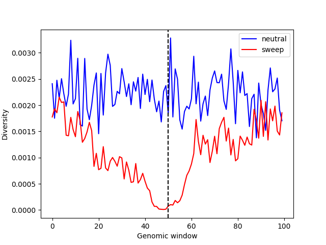
Plot with nucleotide diversity along the chromosome for simulations with a without a selective sweep.

We can see that diversity is substantially reduced around the beneficial mutation (vertical dashed line), relative to what would be expected under neutrality.

5. Using a DFE from one species in another species

There are not very many empirically estimated DFEs in the literature (certainly not as many as demographic models!). How, then, to add selection to your simulation of a species without a published DFE? By diving into the API you could build one yourself. However, it’s easier to borrow one from another species, and arguably biologically more plausible. (At least some aspects of the DFE should be shared at least by some species, such as the swath of deleterious mutations due to breakages in cellular machinery.) For some discussion of this, see Kyriazis et al 2022, which proposes a “generic” DFE for use in a variety of contexts. This DFE was estimated from human data, so it’s under HomSap:

homsap = stdpopsim.get_species("HomSap")
dfe = homsap.get_dfe("Mixed_K23")
print(dfe.long_description)

Even though the DFE is stored under HomSap in the catalogue, we can apply it to a contig from any species. For instance, we could apply it to the first 100Kb of the Vaquita chromosome 1:

vaquita = stdpopsim.get_species("PhoSin")
contig = vaquita.get_contig("1", right=1e5)
contig.add_dfe(intervals=[[0, 1e5]], DFE=dfe)
model = vaquita.get_demographic_model("Vaquita2Epoch_1R22")
samples = {"Vaquita": 50}

engine = stdpopsim.get_engine("slim")
ts = engine.simulate(
    model,
    contig,
    samples,
    seed=159,
    slim_scaling_factor=10,
    slim_burn_in=10,
)

To make the example quick, we’ve only simulated the first 100Kb; a more realistic example would apply it to the exons, available as a annotation.

Tips, tricks, and gotchas

Here are a few things about the whole process that it might be useful to know. Maybe this will save you some time, or let you do new things!

Missing data and coordinates

Suppose as above that we’ve simulated just a portion of a chromosome, using the left and right arguments to species.get_contig( ):

species = stdpopsim.get_species("HomSap")
model = species.get_demographic_model("Africa_1T12")
contig = species.get_contig(
    "chr22", left=10e6, right=20e6, mutation_rate=model.mutation_rate
)
samples = {"AFR": 100}
engine = stdpopsim.get_engine("msprime")
ts = engine.simulate(model, contig, samples)
print(
    f"Sequence length: {ts.sequence_length}\n"
    f"  First variant: {ts.sites_position[0]}\n"
    f"   Last variant: {ts.sites_position[-1]}\n"
)
# Sequence length: 50818468.0
#   First variant: 10000142.0
#    Last variant: 19999926.0

We would like the output to preserve the coordinate system, so all variants we’d see in a VCF file (for instance) are between 10Mb and 20Mb. (And, if you’re just getting a VCF, then no need to read the rest of this!) However, for the tree sequence to retain the same coordinates, it must start at position 0, and end at the sequence length of human chromosome 22. So, the rest of the tree sequence contains “misssing data”, which is encoded as, basically, a big “tree” where no-one is related to anyone else on those segments (in other words, before 10Mb and after 20Mb).

This can lead to surprising things. For instance, the first tree (the tree describing relationships at position 0 along the sequence) has 200 roots:

t = ts.first()
t.num_roots
# 200

Of course, that’s just one root per sample: in other words, there’s actually no trees on this portion of the genome. If we check all the trees using the root_threshold argument to tskit.TreeSequence.trees(), then we’ll correctly see that in fact all trees have fully coalesced (as they should have, because as discussed above, we have recapitated them):

max([t.num_roots for t in ts.trees(root_threshold=2)])
# 1

To read more about using tree sequences, see tskit’s documentation.

Example analyses with stdpopsim

Calculating genetic divergence

Next we’ll give an example of computing some summaries of the simulation output. The tskit documentation has details on many more statistics that you can compute using the tree sequences. We will simulate some samples of human chromosomes from different populations, and then estimate the genetic divergence between each population pair.

1. Simulating the dataset

First, let’s use the --help-models option to see the selection of demographic models available to us:

$ stdpopsim HomSap --help-models

All simulation models for Homo sapiens

Africa_1B08: African-americans population
     African-American two-epoch instantaneous growth model from Boyko
    et al 2008, fit to the synonymous SFS for the 11 of 15 African
    Americans showing the least European ancestry, using coalescent
    simulations with recombination with the maximum likelihood method
    of Williamson et al 2005; times were calibrated assuming 3e5
    generations since human-chimp divergence and fitting the number of
    synonymous human-chimp differences. Mutation and recombination
    rates were assumed to be the same (1.8e-8).

    Populations:
        African_Americans: African-Americans from Boyko et al 2008

Africa_1T12: African population
     The model is a simplification of the two population Tennesen et
    al. model with the European-American population removed so that we
    are modeling the African population in isolation.
...

This prints detailed information about all of the available models to the terminal. In this tutorial, we will use the model of African-American admixture from Browning et al. (2018). From the help output (or the Catalog), we can see that this model has id AmericanAdmixture_4B18, and allows samples to be drawn from 4 contemporary populations representing African, European, Asian and African-American groups.

Using the --help-genetic-maps option, we can also see what genetic maps are available:

$ stdpopsim HomSap --help-genetic-maps

All genetic maps for Homo sapiens

DeCodeSexAveraged_GRCh36
     This genetic map is from the deCode study of recombination events
    in 15,257 parent-offspring pairs from Iceland. 289,658 phased
    autosomal SNPs were used to call recombinations within these
    families, and recombination rates computed from the density of
    these events. This is the combined male and female (sex averaged)
    map. See https://www.decode.com/addendum/ for more details.

DeCodeSexAveraged_GRCh38
     This genetic map is from the deCode study of recombination events
    in 15,257 parent-offspring pairs from Iceland. 289,658 phased
    autosomal SNPs were used to call recombinations within these
    families, and recombination rates computed from the density of
    these events. This is the combined male and female (sex averaged)
    map. See https://www.decode.com/addendum/ for more details. This
    map is further lifted over from the original GRCh36 to GRCh38
    using liftover. Liftover was performed using the
...

Let’s go with HapMapII_GRCh38. The next command simulates 2 diploid samples of chromosome 1 from each of the four populations, and saves the output to a file called afr-america-chr1.trees. For the purposes of this tutorial, we’ll also specify a random seed using the -s option. To check that we have set up the simulation correctly, we may first wish to perform a dry run using the -D option. This will print information about the simulation to the terminal:

$ stdpopsim HomSap -c chr1 -o afr-america-chr1.trees -s 13 -g HapMapII_GRCh38 -d AmericanAdmixture_4B18 AFR:2 EUR:2 ASIA:2 ADMIX:2 -D
Simulation information:
    Engine: msprime (1.3.3)
    Model id: AmericanAdmixture_4B18
    Model description: American admixture
    Seed: 13
    Population: number_samples (sampling_time_generations):
        AFR: 2 (0)
        EUR: 2 (0)
        ASIA: 2 (0)
        ADMIX: 2 (0)
Contig Description:
    Contig origin: chr1:0-248956422
    Contig length: 248956422.0
    Contig ploidy: 2
    Mutation rate: 2.36e-08
    Recombination rate: 1.1523470111585671e-08
    Genetic map: HapMapII_GRCh38

...

Once we’re sure, we can remove the -D flag to run the simulation (this took around 8 minutes to run on a laptop).

$ stdpopsim HomSap -c chr1 -o afr-america-chr1.trees -s 13 -g HapMapII_GRCh38 \
$    -d AmericanAdmixture_4B18 AFR:2 EUR:2 ASIA:2 ADMIX:2

2. Calculating divergences

We should now have a file called afr-america-chr1.trees. Our work with stdpopsim is done; we’ll now switch to a Python console and import the tskit package to load and analyse this simulated tree sequence file.

import tskit

ts = tskit.load("afr-america-chr1.trees")

Recall that genetic divergence (often denoted \(d_{xy}\)) between two populations is the mean density per nucleotide of sequence differences between two randomly sampled chromosomes, one from each population (and averaged over pairs of chromosomes). Genetic diversity of a population (often denoted \(\pi\)) is the same quantity, but with both chromosomes sampled from the same population. These quantities can be computed directly from our sample using tskit’s tskit.TreeSequence.divergence().

By looking at the documentation for this method, we can see that we’ll need two inputs: sample_sets and indexes. In our case, we want sample_sets to give the list of sample chromosomes (nodes) from each separate population. We can obtain the necessary list of lists like this:

sample_list = []
for pop in range(0, ts.num_populations):
    sample_list.append(ts.samples(pop).tolist())

print(sample_list)

# [[0, 1, 2, 3], [4, 5, 6, 7], [8, 9, 10, 11], [12, 13, 14, 15]]

Note that the samples with node IDs 0 - 3 are from population 0, samples with node IDs 4 - 7 are from population 1 and so on. (Also, the .tolist() in the code above is not necessary; it is only there to make the output simpler.)

The next argument, indexes should give the pairs of integer indexes corresponding to the sample sets that we wish to compute divergence between. For instance, the tuple (0, 2) will compute the divergence between sample set 0 and sample set 2 (so, in our case, population 0 and population 2). We can quickly get all the pairs of indexes as follows:

inds = []
for i in range(0, ts.num_populations):
    for j in range(i, ts.num_populations):
        inds.append((i, j))

print(inds)
# [(0, 0), (0, 1), (0, 2), (0, 3), (1, 1), (1, 2), (1, 3), (2, 2), (2, 3), (3, 3)]

We are now ready to calculate the genetic divergences.

divs = ts.divergence(sample_sets=sample_list, indexes=inds)
print(divs)
# [0.00078192 0.00080099 0.00080262 0.00079789 0.00056527 0.00063978
#  0.00063219 0.00057068 0.00062214 0.00064897]

As a sanity check, this demographic model has population sizes of around \(N_e = 10^4\), and the mutation rate that was used to infer parameters for this model was \(\mu = 2.36 \times 10^{-8}\) (shown in the output of stdpopsim, or found in python with model.mutation_rate), so we expect divergence values to be of order of magnitude \(2 N_e \mu = 0.000472\), but slightly higher because of population structure.

3. Plotting the divergences

The output lists the divergences of all population pairs that are specified in indexes, in the same order. However, instead of simply printing these values to the console, it might be nicer to create a heatmap of the values. Here is some (more advanced) code that does this. It relies on the numpy, seaborn and matplotlib packages.

import numpy as np
import seaborn
import matplotlib.pyplot as plt

div_matrix = np.zeros((ts.num_populations, ts.num_populations))
for pair in range(0, len(inds)):
    pop0, pop1 = inds[pair]
    div_matrix[pop0, pop1] = divs[pair]
    div_matrix[pop1, pop0] = divs[pair]

seaborn.heatmap(div_matrix, vmin=0, square=True)
plt.title("Genetic divergence")
plt.xlabel("Populations", fontweight="bold")
plt.ylabel("Populations", fontweight="bold")
plt.xticks([0.5, 1.5, 2.5, 3.5], labels=["AFR", "EUR", "ASI", "ADM"])
plt.yticks([0.5, 1.5, 2.5, 3.5], labels=["AFR", "EUR", "ASI", "ADM"])
plt.show()

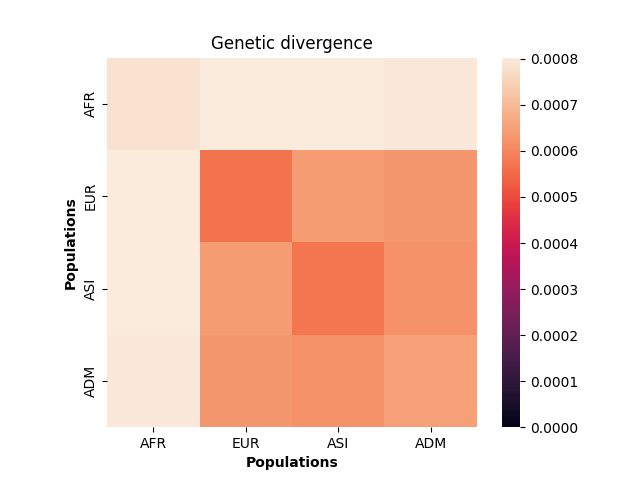
These values make sense given the model of demography we have specified: the highest divergence estimates were obtained when African samples (AFR) were compared with samples from other populations, and the lowest divergence estimates were obtained when Asian (ASI) samples were compared with themselves. However, the overwhelming sameness of the sample chromosomes is also evident: on average, any two sample chromosomes differ at less than 0.07% of positions, regardless of the populations they come from.

Calculating the allele frequency spectrum

Next, we will simulate some samples of chromosomes from different populations of a non-human (finally!), Arabidopsis thaliana, and analyse the allele frequency spectrum (AFS) for each population (also called the “site frequency spectrum, or SFS).

1. Simulating the dataset

This time, we will use the stdpopsim.IsolationWithMigration() model. Since this is a generic model that can be used for any species, we must use the Python interface for this simulation. See our Python tutorial for an introduction to this interface.

We begin by importing stdpopsim into a Python environment and specifying our desired species, Arabidopsis thaliana. From the Catalog, we can see that this species has the ID AraTha:

import stdpopsim

species = stdpopsim.get_species("AraTha")

After skimming the Catalog to see our options, we’ll specify our desired chromosome chr4 and genetic map SalomeAveraged_TAIR10.

contig = species.get_contig("chr4", genetic_map="SalomeAveraged_TAIR10")

From the API description, we can see that the stdpopsim.IsolationWithMigration() model allows us to sample from a pair of populations that diverged from a common ancestral population. We’ll specify that the effective population size of the ancestral population was 5000, that the population sizes of the two modern populations are 4000 and 1000, that the populations diverged 1000 generations ago, and that rates of migration since the split between the populations are both zero.

model = stdpopsim.IsolationWithMigration(
    NA=5000, N1=4000, N2=1000, T=1000, M12=0, M21=0
)

We’ll simulate 5 diploids from each of the populations using the msprime engine (the populations in this generic model are named pop1 and pop2).

samples = {"pop1": 5, "pop2": 5}
engine = stdpopsim.get_engine("msprime")

Finally, we’ll run a simulation using the objects we’ve created and store the outputted dataset in an object called ts. For the purposes of this tutorial, we’ll also run this simulation using a random seed:

ts = engine.simulate(model, contig, samples, seed=13)

2. Calculating the AFS

Recall that the allele frequency spectrum (AFS) summarises the distribution of allele frequencies in a given sample. At each site, there is an ancestral and (sometimes more than one) derived allele, and each allele is observed in the sample with some frequency. Each entry in the AFS corresponds to a particular sample frequency, and records the total number of derived alleles with that frequency. We can calculate the AFS directly from our tree sequence using the tskit.TreeSequence.allele_frequency_spectrum() method.

Since we wish to find the AFS separately for each of our two populations, we will first need to know which samples correspond to each population. The tskit.TreeSequence.samples() method in tskit allows us to find the IDs of samples from each population:

pop_samples = [ts.samples(0), ts.samples(1)]
print(pop_samples)
# [array([0, 1, 2, 3, 4, 5, 6, 7, 8, 9], dtype=int32),
#  array([10, 11, 12, 13, 14, 15, 16, 17, 18, 19], dtype=int32)]

We are now ready to calculate the AFS. Since our dataset was generated using the default msprime simulation engine, we know that it has exactly one derived allele at any polymorphic site. We also know what the derived and ancestral states are. We can therefore calculate the polarised AFS using tskit’s tskit.TreeSequence.allele_frequency_spectrum() method:

sfs0 = ts.allele_frequency_spectrum(
    sample_sets=[pop_samples[0]], polarised=True, span_normalise=False
)
print(sfs0)
# [1686. 2496. 1232.  850.  614.  566.  456.  396.  309.  322.  123.]

The output lists the number of derived alleles that are found in 0, 1, 2, … of the given samples. Since each of our populations have 10 samples each, there are 11 numbers. The first number, 1686, is the number of derived alleles found in the tree sequence but not found in that population at all (they are present because they are found in the other population). The second, 2496, is the number of singletons, and so forth. The final number, 123, is the number of derived alleles in the tree sequence found in all ten samples from this population. Since an msprime simulation only contains information about polymorphic alleles, these must be alleles fixed in this population but still polymorphic in the other.

Here is the AFS for the other population:

sfs1 = ts.allele_frequency_spectrum(
    sample_sets=[pop_samples[1]], polarised=True, span_normalise=False
)
print(sfs1)
# [3790. 1021.  729.  583.  522.  455.  386.  335.  285.  264.  680.]

The somewhat mysterious polarised=True option indicates that we wish to calculate the AFS for derived alleles only, without “folding” the spectrum, and the span_normalise=False option disables tskit’s default behaviour of dividing by the sequence length. See tskit’s documentation for more information on these options.

We will do further analysis in the next section, but you might first wish to convince yourself that this output makes sense to you. You might also wish to check that the total number of mutations is the sum of the AFS entries:

sum(sfs0), sum(sfs1), ts.num_mutations
# (9050.0, 9050.0, 9050)

3. Plotting the AFS

Here is some more advanced code that compares the estimated AFS from each population. It relies on the matplotlib and numpy packages. We will scale each AFS by the number of mutated sites in the corresponding sample set.

import matplotlib.pyplot as plt
import numpy as np

bar_width = 0.4
r1 = np.arange(0, 11) - 0.2
r2 = [x + bar_width for x in r1]
plt.bar(x=r1, height=sfs0 / ts.num_sites, width=bar_width, label="pop0")
plt.bar(x=r2, height=sfs1 / ts.num_sites, width=bar_width, label="pop1")
plt.xlabel("Allele count", fontweight="bold")
plt.ylabel("Proportion of mutated sites in sample", fontweight="bold")
plt.xticks(np.arange(0, 11))
plt.legend()
plt.show()

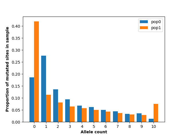
This figure shows substantial differences in the allele frequency spectrum between the two populations, most notably a larger number of singletons in population 0 and a larger number of fixed and absent alleles in population 1. This makes sense given the demography we have specified: population 1 has had a much more extreme population size reduction.

Tutorials

Running stdpopsim with the command-line interface (CLI)

A first simulation

Choose a species and a contig

Choose a model and a sampling scheme

Convert output to VCF

Using the SLiM simulation engine

Specifying the engine

SLiM scaling factor

Simulating genomes with selection

Debugging output from SLiM

Choose a species: Drosophila melanogaster

Running stdpopsim with the Python interface (API)

Running a published model

Pick a species and demographic model

Set up the contig

Choose a sampling scheme and simulate

Running a generic model

Choose a species

Set up the generic model

Choose a contig and genetic map

Choose a sampling scheme, and simulate

Sanity check the tree sequence output

Output to VCF

Using the SLiM engine

An example simulation

Choose the species, contig, and genetic map

Choose the simulation engine

Other SLiM options

The SLiM burn-in

Outputting the SLiM script

Incorporating selection

1. Simulating with a genome-wide DFE

2. Simulating selection in a single gene

3. Simulating selection on exons

4. Selective sweeps

5. Using a DFE from one species in another species

Tips, tricks, and gotchas

Missing data and coordinates

Example analyses with stdpopsim

Calculating genetic divergence

1. Simulating the dataset

2. Calculating divergences

3. Plotting the divergences

Calculating the allele frequency spectrum

1. Simulating the dataset

2. Calculating the AFS

3. Plotting the AFS

Using the `SLiM` simulation engine

`SLiM` scaling factor

Debugging output from `SLiM`

Using the `SLiM` engine

Other `SLiM` options

The `SLiM` burn-in

Outputting the `SLiM` script